Benchmark

Wall time of a single classical fourth-order Runge-Kutta step of the pseudo-spectral Navier-Stokes solver (benchmarks/bench_workload.py, Taylor-Green initial condition), across log-spaced 3D grid sizes. Lower is better.

Test machine & code version

• CPU: AMD Instinct MI300A Accelerator (192 logical cores)
• GPU: 4x AMD Instinct MI300A
• muNavierStokes: dcc04b3 — run 2026-06-24T15:13:45

Run configuration: triply-periodic box, kinematic viscosity ν = 1/1600, time step 1e-3, 2/3-rule dealiasing on. Each data point times 20 RK4 steps (after warm-up) and reports the mean — i.e. a fixed work budget, so every configuration performs identical arithmetic. Timing covers only the integration loop (no file I/O, no diagnostics). One RK4 step evaluates the right-hand side four times; each evaluation runs several 3-component forward/inverse FFTs plus the fused per-pixel curl, dealiasing, viscous, and Leray-projection kernels.

Time vs. grid size

The plot below merges the ways of running the same solver on this machine:

• CPU (1 core) — a single core, MPI disabled (the non-MPI muGrid build). muGrid's compute kernels carry no OpenMP, so a non-MPI CPU run uses one core.
• CPU (92 cores, MPI) — the whole CPU via MPI pencil decomposition (mpiexec -n 92), the grid split into per-rank subdomains whose FFTs exchange data each transform.
• GPU (1 device) — the whole GPU (cuFFT plus the fused device kernels).
• GPU (N devices, MPI) — all GPUs, one rank per device.

Configuration	32³ (33k)	48³ (111k)	64³ (262k)	96³ (885k)	128³ (2.1M)	192³ (7.1M)	256³ (16.8M)	512³ (134.2M)
CPU (1 core)	8.27	44	95	418	1.1e+03	3.39e+03	8.01e+03	6.5e+04
CPU (92 cores, MPI)	2.59	5.27	7.05	20.7	38.7	146	280	2.67e+03
GPU (1 device)	3.13	3.23	2.92	3.7	6.84	17	48	—
GPU (4 devices, MPI)	4.29	5.16	10.3	15.5	32.9	98	227	—

(values are milliseconds per RK4 step)

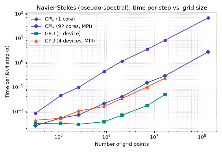
The workload is dominated by the multidimensional FFTs, which are memory-bandwidth-bound, so the time tracks memory throughput rather than peak FLOPs. Two regimes are visible. At small grids the GPU is overhead-bound: a fixed per-step cost of kernel launches and host/device synchronisation (a few milliseconds) dominates, so the GPU is actually the slowest configuration while the single CPU core, with almost no fixed overhead, wins on the tiniest grids. Past the crossover (here around \(10^5\) grid points) the picture flips: the GPU's high memory bandwidth takes over and it becomes the fastest by a growing margin, while the full CPU via MPI sits in between — well ahead of one core but short of the GPU.

Multi-GPU

The solver binds each MPI rank to the communicator it is given, so on a host with several GPUs mpiexec -n <#GPUs> python bench_workload.py -d cuda runs one rank per device. This benchmark adds a GPU (N devices, MPI) curve automatically when more than one GPU is present. This run used several GPUs, so the multi-GPU curve is shown.

MPI strong scaling (CPU)

Strong scaling of the same step (fixed problem size, increasing MPI ranks) on the 92-core CPU.

96³ (884,736 points)

Ranks	ms/step	Speedup	Parallel eff.
1	413.53	1.00×	100%
2	380.82	1.09×	54%
4	215.73	1.92×	48%
8	132.52	3.12×	39%
16	49.10	8.42×	53%
32	23.71	17.44×	54%
64	20.17	20.50×	32%
92	21.13	19.57×	21%

128³ (2,097,152 points)

Ranks	ms/step	Speedup	Parallel eff.
1	1103.72	1.00×	100%
2	994.89	1.11×	55%
4	570.58	1.93×	48%
8	374.19	2.95×	37%
16	165.27	6.68×	42%
32	71.17	15.51×	48%
64	37.93	29.10×	45%
92	39.49	27.95×	30%

192³ (7,077,888 points)

Ranks	ms/step	Speedup	Parallel eff.
1	3407.55	1.00×	100%
2	3120.94	1.09×	55%
4	1809.77	1.88×	47%
8	1302.92	2.62×	33%
16	650.18	5.24×	33%
32	332.79	10.24×	32%
64	156.09	21.83×	34%
92	163.47	20.84×	23%

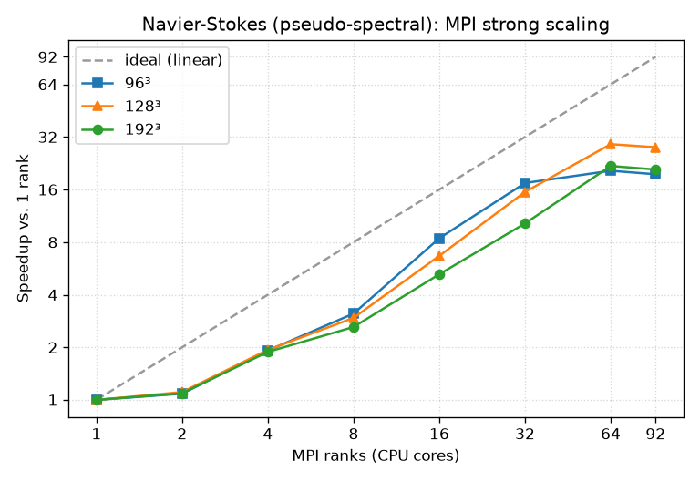
Scaling is strong at low rank counts and then tapers: the pseudo-spectral step is memory-bandwidth-bound and the distributed FFT needs an all-to-all transpose each transform, so once per-rank subdomains get small the transpose communication and the CG-style reductions begin to dominate. Larger grids keep scaling further because they keep more work per rank.

All data points live in the shared benchmark database benchmarks/results.csv (date, code version, machine, parameters, results). This page is generated by benchmarks/benchmark.py; re-render it from the database (no recompute) with --render-only, or run a fresh measurement that appends a new dated row set:

python benchmarks/benchmark.py --doc-out docs/benchmark.md